Matlab è un ambiente destinato al calcolo numerico, alla simulazione e allo sviluppo di modelli matematici. Il linugaggio Matlab è dinamico; i tipi base non sono valori scalari, bensì matrici. Il codice è JIT-compilato, la memoria è gestita da un garbage collector.
Durante la preparazione dell'esame di Analisi 2 - presso il Politecnico di Milano - ho sviluppato questa semplice routine per il calcolo e la rappresentazione della serie di Fourier associata ad una funzione. La pubblico con la speranza che possa essere utile ad altri studenti e interessare chi non ha mai utilizzato l'ambiente Matlab.
%
% DRAWFOURIER
%
% Definition:
% function [xvalues, yvalues] = drawfourier(y, x, from, to, step, precision)
%
% Description:
% Draws the graphic of the function y(x) and the graphic of its Fourier's
% series. Requires the Symbolic Math Toolbox.
%
% Arguments:
% y: symbolic expression of the function
% x: symbolic variable rappresenting the independent variable
% from: left boundary of the period
% to: right boundary of the period
% step: the distance beetween two points in which the series is computed
% precison: the maximum index of the series
%
% Returned values:
% xvalues: the values in the domain of the Fourier's series
% yvalues: the values of the Fourier's series
%
% Example:
% x = sym('x'); drawfourier(x^2, x, -pi, pi, 0.1, 50);
%
% Information:
% Author: Andrea Sansottera (andrea.sansottera@fastwebnet.it)
% Date: June 20th 2005
% Version: 0.6
% License: GPL
function [xvalues, yvalues] = drawfourier(y, x, from, to, step, precision)
% starts the stopwatch
tic;
% initializes the symbolic index of the series
k = sym('k');
% initializes period and pulsation
t = (to - from);
c = 2/t;
omega = (2*pi)/t;
% computes the Fourier coefficients of the series
a0 = c * int (y, from, to);
ycos = y * cos(omega*k*x);
ak = c * int(ycos, from, to);
ysin = y * sin(omega*k*x);
bk = c * int(ysin, from, to);
% defines the domain of the series
xvalues = [from : step : to];
% foreach point in the domain of the function
for i = [1 : length(xvalues)]
% computes the value of the Fourier's series
yvalues(i) = subs(a0/2);
for kval = 1 : precision
yvalues(i) = yvalues(i) + subs(ak*cos(omega*k*x), {k, x}, {kval, xvalues(i)});
yvalues(i) = yvalues(i) + subs(bk*sin(omega*k*x), {k, x}, {kval, xvalues(i)});
end
end
% plots the function
ezplot(y, [from, to]);
% keeps the graphic on the figure
hold on;
% plots the Fourier's series
plot(xvalues, yvalues, 'r');
% sets the labels of the figure
xlabel('x');
ylabel('y');
% sets the title of the figure
figure_title = sprintf('%s period = [%.2f, %.2f] step = %.2f k = [1, %d]', char(y), from, to, step, precision);
title(figure_title);
% displays a legend
series_label = sprintf('Fourier''s series of %s', [char(y)]);
legend(char(y), series_label);
% setups axis
axis([from to min(yvalues) max(yvalues)]);
% stops the stopwatch and displays the elapsed time
toc;
end
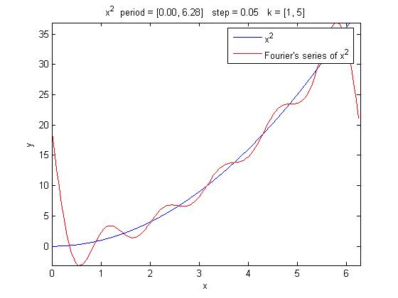
Ecco un esempio. Disegniamo la parabola di equazione x^2 e la sua serie di Fourier, nell'intervallo [0, 2*pi], valutandola ogni 0.05. Consideriamo solamente i primi 5 termini della serie.
syms x; drawfourier (x^2, x, 0, 2*pi, 0.05, 5)
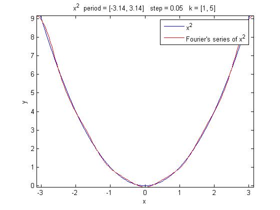
Essendo la funzione limitata e monotona a tratti, sono soddisfatte le ipotesi del teorema di convergenza puntuale. Cerchiamo di sfruttarlo per ottenere una migliore approssimazione. Scegliamo un intervallo in cui la funzione presenti simmetria pari: in tale intervallo soddisferà la condizione di raccordo. Poichè la funzione è continua la serie di Fourier converge in ogni singolo punto alla y(x). Si noti come in questo modo l'approssimazione migliori, pur sottoponendo la macchina allo stesso carico computazionale (il termini valutati sono sempre i primi 5).
syms x; drawfourier (x^2, x, -pi, +pi, 0.05, 5)
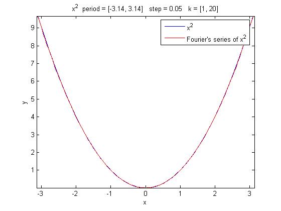
Com'è facilmente intuibile, aumentando il numero di termini della serie valutati, la precisione migliora ulteriormente.
syms x; drawfourier (x^2, x, 0, 2*pi, 0.05, 20)